This shows that with upslope winds, the data is influenced by local CO2
depleted air. These data are rightfully discarded from the
daily/monthly/yearly averages, as they don't reflect the background CO2
levels, which we are interested in.
Does discarding of "contaminated" data influence the trend over a year
or several years? I have asked that question to Pieter Tans,
responsible for dataprocessing of the Mauna Loa data. His answer:
The
data selection method has been described in Thoning et al., J. Geophys.
Research, (1989) vol. 94, 8549-8565. Different data selection
methods are compared in that paper, including no selection. The methods give annual means differing by
a few tenths of 1 ppm. I assume that you have read the
README file [
4]
when downloading the data. The
hourly means are NOT pre-processed, but they are flagged when the
st.dev. of the minute averages is large.
The good, the bad and the ugly
stations.
Several stations are deemed "good", as these have minimal influence
from local vegetation and/or human emissions (traffic, heating). These
are stations in the middle of the oceans, sometimes at coastal points
(as long as the wind is not blowing from land side) and/or above the
inversion layer. These stations, after discarding outliers, differ from
each other within 5 ppmv for yearly averages, of which most is from the
delay between the NH and the SH, see next item. 10 of them, spanning
the
globe from near the North Pole (Alert, Canada) to the South Pole, are
used as reference for daily, monthly and yearly averages and yearly
trends. The graphs and the data can be found at [
5].
Some inland stations, like Schauinsland only give reliable "background"
CO2
levels, when the station (at 1200 m altitude) is above the inversion
layer and with enough wind speed. This happens only about 10% of the
time.
And last, but not least, many inland stations are practically
unsuitable for background CO2 measurement, because of incomplete mixing
with the higher air layers, partly due to too many local sources/sinks
like vegetation and/or human use of fossil fuels, partly due to a
shielded location. This is the case for e.g. Diekirch (Luxemburg) [
6],
where the station is in a valley with forests,
urbanisation and traffic in the main upwind direction:

Diekirch (Luxemburg) CO2 measurements compared to wind speed
Graph from [
6].
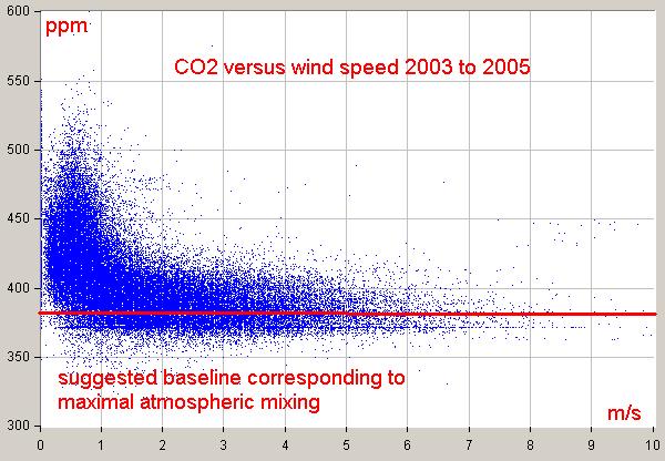
As can be seen, even at inconvenient places with lots of local
sources/sinks, there is an inverse correlation between CO2 levels and
wind speed. With higher wind speeds, CO2 levels are better mixed with
higher air layers which have "background" CO2 content. This reduces the
CO2 content at ground level. The assymptote of CO2 levels at high speed
winds (as was seen during storm Franz, 11 January 2007) is about 385
ppmv, very close to the 382 ppmv level found at Mauna Loa in the same
period. The same is true for diurnal variance: at daytime and with high
enough wind speed (> 1 m/s), CO2 levels are lower and near
background, while at night under the inversion layer, CO2 levels are up
to 100 ppmv higher.
3. Variations
of
CO2 due to the seasons:
There are two main natural influences on the CO2 levels of the
atmosphere: the temperature of the ocean's surface waters and the
uptake of CO2 by plants in spring/summer and the release of CO2 by the
decay of dead plant material in fall/winter. This is most clear in the
NH (Northern Hemisphere), where most of vegetation on land is situated.
CO2 is continuously emitted by deep sea upwelling, especially in the
tropics, where temperatures are high and the partial pressure of CO2
(pCO2) in the upper oceans is higher than in the atmosphere above it.
CO2 is continuously absorbed in the upper ocean layers at higher
latitudes, where the colder temperatures reduce the pCO2 of the oceans,
lower than the pCO2 of the atmosphere. This is especially the case at
the sink places of the THC (thermohaline circulation) in the Nordic
Atlantic ocean. Colder water can retain more CO2 than warmer water, but
in the case of CO2 there are also a lot of chemical and biological
reactions which influence the solubility of CO2 and hence pCO2 at the
surface of the oceans. For more details on this,
Wiki has a
quite good explanation.
The CO2 flow between the tropics and the colder places in the oceans is
relatively constant (more about that later), and doesn't influence the
seasonal variation that much. More variation is in the temperature (and
thus pCO2) of the mid-latitudes, where there is absorption of CO2 in
winter and release of CO2 in summer. The CO2 flow of vegetation
(including algues in the upper oceans) is in opposite direction: more
release in winter and more uptake in summer. The net effect in the NH
is a
variation of +/-4 ppmv in Mauna Loa (mid Pacific Ocean, middle
troposphere) between summer and winter, up to +/-20 ppmv for Barrow
(Alaska, USA, sea level, near tundra) or even 35 ppmv at Schauinsland
(Germany, 1200 m high). The data of
Schauinsland are heavily contaminated by the nearby fully inhabited and
industrialised Rhine valley. And influenced by vegetation, in this case
the Black Forest of SW Germany. Only at night, when separated from the
valleys by an inversion layer, and with sufficient wind speed, the CO2
levels are better mixed with the rest of the troposphere and retained.
This is the case for only 10% of the data.
Data series from the SH (Southern Hemisphere) show much less seasonal
variation, because of the much smaller area of land/vegetation. The
smallest influence of the seasons is found at the South Pole.
Here follows some comparison of the Mauna Loa (selected) monthly
averages with these of other stations:

Monthly trends 2002-2004 of 2 NH stations (Barrow and Mauna Loa) and 2
SH stations (Samoa and South Pole)
As can be noticed, the variation at Mauna Loa is smaller than at Barrow
and the SH stations have a much smaller seasonal influence than the NH
stations. Also, although the trend of the SH stations is near the same,
there is some lag between the NH and SH stations. This is the first
indication that the source of the increase is situated in the NH, as
the ITCZ (intertropical convergence zone) forms a barrier for the
exchange of CO2 (and aerosols) between the NH and the SZ. This is even
more clear in the longer term yearly trends:

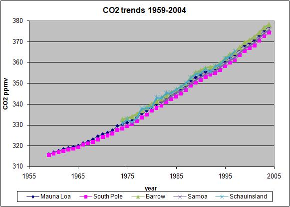
Trends in yearly averages of CO2 levels at different stations.
The trend of the SH stations has a growing delay of 6-12 months behind
the NH trend. But all yearly average data of the "best" stations (and
the average of least contaminated data from less suitable stations like
Schauinsland) are within 5 ppmv for similar growth.
4. Where to measure? The concept of
"background" CO2 levels.
The concept was launched by C.D. Keeling in the mid fifties, when he
made several series of measurements in the USA. He found widely varying
CO2 levels, sometimes in samples taken as short as 15 minutes from each
other. He also noticed that values in widely different places, far away
from each other, but taken in the afternoon, were much lower and much
closer resembling each other. He thought that this was because in the
afternoon, there was more turbulence and the production of CO2 by
decaying vegetation and/or emissions was more readily mixed with the
overlying air. Fortunately, from the first series on [
2],
he also measured 13C/12C ratios of the same samples, which did prove
that the diurnal variation was from vegetation decay at night, while
during the day photosynthesis at one side and turbulence at the other
side increased the 13C/12C ratio back to maximum values.
Keeling's first series of samples, taken at Big Sur State Park, showing
the diurnal CO2 and d13C cycle was published in [
7],
original data (of other series too) can be found in [
8]:
Figure 3.1 Diurnal variation in the concentration and carbon
isotopic ratio of atmospheric
CO
2 in a coastal redwood forest of California, 18-19 May
1955, Big Sur St. Pk.
(Keeling, 1958. Reproduced by permission of Pergamon Press.)
Several others measured CO2 levels/d13C ratios of the their own samples
too. This happened at several places in Germany (Heidelberg,
Schauinsland, Nord Rhine Westphalia). This confirmed that local
production was the origin of the high CO2 levels. The smallest CO2/d13C
variations were found in mountain ranges, deserts and near the oceans.
The largest in forests, urban neighbourhoods and non-urban, but heavely
industrialised neighbourhoods. When the reciproke of CO2 levels were
plotted against d13C ratios, this showed a clear relationship between
the two. Again from [
7]:

Figure 3.5 Relation between carbon isotope ratio and concentration of
atmospheric CO
2 in
different air types from measurements summarized in Table 3.4
(Keeling, 1958, 1961: full squares; Esser, 1975: open circles; Freyer
and Wiesberg, 1975,
Freyer, 1978c: open squares). All
13C measurements have not been
corrected
for N
2O contamination (Craig and Keeling, 1963), which is at
the most in the area of + 0.6‰
The
search for background places.
Keeling then sought for places on earth not (or not much) influenced by
local production/uptake, thus far from forests, agriculture and/or
urbanisation. He had the opportunity to launch two continuous
measurements: at Mauna Loa and at the South Pole. Later, other basic
stations were added, all together 10 from near the North Pole (Alert,
NWT, Canada) to the South Pole, most of them working continuous, some
working with regular flask sampling.
We are interested in CO2 levels in a certain year all over the globe
and the trends of the CO2 levels over the years. So, here we are at the
definition of the "background" level:
Yearly average data taken from places minimal influenced by vegetation
and human sources are deemed "background".
For convenience, the yearly average data from Mauna Loa are used as
reference. One could use any base station as reference or the average
of the stations, but as all base stations (and a lot of other stations,
even Schauinsland) are within 5 ppmv of Mauna Loa, with near identical
trends, and that station has the longest near-continuous CO2 record,
Mauna Loa is the
reference.
As the oceans represent about 70% of the earth's surface, and all
oceanic stations show near the same yearly averages and trends, already
70% of the atmosphere shows background behaviour (within 5 ppmv). This
can be extended to near the total earth for the part above the
inversion layer.
Measurements above the inversion layer.
Above land, diurnal variations are only seen up to 150 m (according to [
7]).
Seasonal changes reduce with altitude. This is based on years of
flights (1963-1979) in Scandinavia [
7] and between
Scandinavia and California [
9]. Further confirmed by
old and modern [
10] flights in the USA and Australia
(Tasmania). In the SH, the seasonal variation is much smaller and there
is a high-altitude to lower altitude gradient, where the high altitude
is 1 ppmv richer in CO2 than the lower altitude. This may be caused by
the supply of extra CO2 from the NH via the southern branch of the
Hadley cell to the upper troposphere in the SH.
From [
7], based on [
9]:
Figure 3:2 Amplitude and phase shift of seasonal variations in
atmospheric CO
2
at different altitudes, calculated from direct observations by harmonic
analysis
(Bolin and Bischof, 1970. Reproduced by permission of the Swedish
Geophysical Society.)
From [
10]:

Modern flight measurements in Colorado, CO2 levels below the inversion
layer
in forested valleys and above the inversion layer at different
altitudes
As one can see, again the values above the inversion layer are near
straight and agree within a few ppmv with the Mauna Loa data. Below the
inversion layer, the morning values are 15-35 ppmv higher, in the
afternoon, these may sink to background again.
If we take the 1000 m as the average upper level for the influence of
local disturbances, that represents about 10% of the atmospheric mass.
Thus the "background" level can be found at 70% of the earth's air mass
(oceans) + 90% of the remaining land surface (27%). That is in 97% of
the global air mass. Only 3% of the global air mass contains not-well
mixed amounts of CO2, which is only over land.
General conclusion:
Background CO2 levels can be found
over all oceans and over land at 1000 m and higher altitudes (in
high mountain ranges, this may be higher).
5. Evidence of human
influence on the increase of CO2 in the atmosphere.
5.1.
The
mass balance
The amount of CO2 emitted by humans nowadays is about 7 GtC/yr (CO2
counted as carbon). The increase in the atmosphere is about 4 GtC/yr.
That implies that there is little to no increase in the atmosphere due
to other causes, or the amount in the atmosphere in the case of a
natural unbalance should be higher than the emissions, not lower. To
show this for the past near 50 years [
11]:

The graph shows the increase in CO2 from emissions, land use and others
vs. the increase found
in the atmosphere, land and oceans, expressed in GtC/yr
The graph is based on calculations of emissions, sampled from national
inventories of fuel use and land use change. In the best case, these
are accurate, in the worst case, the emissions are underestimated (as
probably is the case for China). Inventories of the atmosphere are
based on very accurate measurements of CO2 at Mauna Loa. The difference
between CO2 emissions (expressed in gigaton carbon per year - GtC/yr)
and carbon increase in the atmosphere is what the oceans and/or
vegetation absorb each year. The partitioning between land and ocean as
sinks is not accurately known, but not of interest here,
as in every year the sum of
land+oceans is more sink than source.
Some investigations were done to know the sink partitioning
between land and oceans by Battle ea. [
12], based on
changes of d13C and oxygen content in the atmosphere over the last
decade of the previous century and earlier estimates:
The increase of CO2 in the atmosphere of about 60 ppmv (122
GtC) in the past near 50
years is about 60% of the increase since the start of the industrial
revolution. This is based on accurate measurements at Mauna Loa and a
lot of other places. The amount of CO2 in the atmosphere in
pre-industrial times is based on ice cores, which of course are less
certain and more smoothed, but there are other proxies with a better
resolution in time, which point to lower CO2 levels prior to the
emissions.
As the first graph shows, in any year of the past near 50 years, the
emissions
are larger than the increase in the atmosphere. That means that the
total mass balance of all natural variables (temperature, ocean pH,
vegetation) which influence CO2 levels, is always towards more sink
than source over any year:
Csources + Cemissions = Csinks + dCair
where Cemissions = 2.5 (1960) to 7 GtC/yr (2006) and increasing
and dCair = 1 (1960) to 6 GtC/yr (2006) and increasing in ratio with
55% of the
emissions
and Csinks = Csources + 1.5 (1960) to 4 GtC (2006) +/- 2 GtC (natural
variability), where the sink capacity
increases in ratio with about 45% of the emissions, while the natural
variability around the trend seems not increasing or decreasing. The
natural variability in sink capacity seems mainly temperature dependent
with a ratio of about 4 ppmv/
°C, based on temperature/CO2 changes during the 1992
Pinatubo eruption and the 1998 strong El Niño. This is
short-term variability around the trend. Over (very) long periods of
time (Vostok ice core), the influence of temperature on CO2 levels is
about 8 ppmv/°C.
The natural seasonal exchange between vegetation and oceans at one side
and the atmosphere at the other side is estimated at about 150 GtC/yr.
But that is not of interest for what the change is over a year, as most
of the natural releases are absorbed within the same year. The
difference after a year is not more than +/- 2 GtC, mainly caused by
temperature changes (El Niño, Pinatubo eruption). Thus the
natural variations over a year are smaller than the emissions. No
matter how high the natural seasonal turnover might be, in all
years over the previous near 50 years, the natural CO2 sinks were
larger than the
natural CO2 sources... Thus it is impossible that natural sources were
responsible for (a substantial part of) the increase of CO2 in the past
50 years.
This proves beyond doubt that human
emissions are the main cause of the increase of CO2, at least
over the past near 50 years. But there are much more indications for
that...
5.2. The process
characteristics:
Here is a graph of the (global) temperature trend, the
cumulative amount of emissions and the increase of CO2 in the
atmosphere (1900-2004):
The temperature trend is for the sea surface,
according to the Hadley Centre in the UK. The emissions are from the
international inventory data base. And the CO2 in the atmosphere
pre-1959 are from ice cores (Law Dome, Siple Dome), from 1959 on, the
data are taken at Mauna Loa (Hawai). Baseline of the CO2 level is 300
ppmv. The 21 year moving average is added, as some have found a good
correlation between that average and the CO2 increase. That is right
after 1980 (where the correlation was based on), but fails for the
whole 1900-2004 period.
As one can calculate, the correlation between temperature and CO2
levels in
the atmosphere is rather weak (corr.: 0.843; R^2: 0.711), and
from the detailed T/dCO2 graphs, one can see that a huge change in
temperature in a certain year has little influence on CO2 levels,
compared to the
influence of the
temperature change over the whole trend.:
This indicates that temperature is not the cause of the trend, but the
cause of the variation (+/- 1.2 ppmv) around the trend (currently over
1.5 ppmv/yr). More about that is coming (if I had only 36 hours in a
day)...
At the other side, the correlation between cumulative emissions and
increase in
the atmosphere is a near-fit (corr.: 0.998; R^2: 0.997) over the whole
period:
The ratio is about 0.53% between increase in the atmosphere and
what is emitted. This points to a simple linear first order process,
directly related to the partial pressure difference between CO2 in the
atmosphere and CO2 in the oceans (and vegetation). The higher the CO2
content in the atmosphere, the higher the push to drive CO2 into the
oceans. Currenty, the partial pressure difference (pCO2) between the
atmosphere and the oeans is about 7 ppmv [
18], based on ship's
surveys and
buoys. The increase of the pCO2 difference causes more and more uptake
of CO2 by the oceans (and
similarly in vegetation).
Again, this clear relationship points to a direct influence of the
emissions on the increase in the atmosphere. There is no known natural
process that is able to force CO2 into the atmosphere exactly in the
same ratio as is the case here for the emissions. One only need to look
at the difference in variability of the temperature curve (which has a
limited influence on CO2 levels of about 4 ppmv/
°C) with the smoothness of the emissions curve...
This adds to the weight of the
emissions as main cause of the increase in the atmosphere.
5.3. The 13C/12C ratio:
The carbon of CO2 is composed
of different isotopes. Most is of the lighter type: 12C (that has 6
protons and 6 neutrons in the kernel), and about 1.1% is heavier: 13C
(has 6 protons and 7 neutrons in the kernel). There also is some 14C (6 protons and 8 neutrons in the kernel),
which is continuously formed in the upper stratosphere from the
collisions of nitrogen with cosmic rays particles. This type of carbon
(also formed by above-ground atomic bomb experiments in the 1950's) is
radio-active and can be used to determine the age of fossils up to
about 60,000 years.
One can measure the 13C/12C ratio and compare it to a standard. The
standard was some type of carbonate rock, called Pee Dee Belemnite
(PDB). When the standard rock was exhausted, this was replaced by a
zero definition in a Vienna conference, therefore the new standard is
called the VPDB (Vienna PDB). Every carbon containing part of any
subject can be measured for its 13C/12C ratio. The comparison with the
standard is expressed as d13C in per mille:
(13C/12C)sampled
– (13C/12C)standard
——————————––––––––––––––– x 1.000
(13C/12C)standard
Where the standard is defined as 0.0112372 part of 13C to 1 part of
total carbon. Thus positive values have more 13C, negative values have
less 13C. Now, the interesting point is that vegetation growth in
general uses by preference 12C, thus if you measure d13C in vegetation,
you will see that it has quite low d13C values. As fossil fuels were
formed from vegetation (or methanogenic bacteria, with similar
preferences), these have low d13C values too. Most other carbon
sources (oceans, carbonate rock wearing, volcanic outgassing,...) have
higher d13C values. For a nice introduction of the isotope cycle in
nature, see the web page of
Anton Uriarte Cantolla [13].
This is an interesting feature, as we can determine if CO2
levels in the atmosphere (which is at -8 per mille VPDB) were
influenced
by vegetation decay or fossil fuel burning (both about -24 per mille)
at
one side (towards the negative side) or by ocean degassing (0 to +4 per
mille) towards the positive side as largest possible sources.
From different CO2 base stations, we not only have CO2 measurements,
but also d13C measurements. Although only over a period of about 25
years, the trend is clear and indicates an extra source of low d13C in
the atmosphere.

Recent trends in d13C from direct measurements of ambient air at 10
base stations. Data from [
14].
ALT=Alert; BAR=Barrow; LJO=La Jolla; MLO=Mauna Loa; CUM=Cape Kumukahi;
CHR=Christmas Island;
SAM=Samoa; KER=Kermadec Island; NZD=New Zealand (Baring Head);
SPO=South Pole.
Again, we see a lag in the trends with
altitude and NH/SH border transfer and less variability in the SH.
Again, this points to a source in the NH. If that is from vegetation
decay (more present in the NH than in the SH) and/or from fossil fuel
burning (90% in the NH) is solved in the investigation of Battle ea. [
12], where it is shown that there
is less oxygen used than can be calculated from fossil fuel burning.
Vegetation thus produces O2, by incorporating more CO2 than is formed
by decaying vegetation (which uses oxygen). This means that more 12C is
incorporated, and thus more 13C is left behind in the atmosphere.
Vegetation is thus a source of 13C and is not the cause of decreasing
d13C ratio's.
And we have several other, older measurements of d13C in the
atmosphere: ice cores and firn (not completely closed air bubbles in
the snow/ice). These align smoothless with the recent air measurements.
There is a similar line of measurements from coralline sponges and
sediments in the upper oceans. Coralline sponges grow in shallow waters
and their sceleton is built from CO2 in the upper ocean waters, without
altering the 13C/12C ratio in seawater at the time of building. The
combination of atmospheric/firn/ice and ocean measurements gives a nice
history of d13C changes over the past 600 years:

Figure from [
15] gives a comparison of upper ocean
water and atmospheric d13C changes.
What we can see, is that the d13C levels as well as in the atmosphere
as in the upper oceans start to decrease from 1850 on, that is at the
start of the industrial revolution. In the 400 years before, there is
only a small variation, probably caused by the temperature drop in the
Little Ice Age.
Again this is a good indication of the
influence of
fossil fuel burning...
5.4. The 14C/12C ratio:
14C is a carbon isotope that is made in the atmosphere by the
impact of cosmic rays. It is an unstable (radioactive) isotope and
breaks down with a half-life time of about 6,000 years. 14C is used for
radiocarbon dating of not too old fossils (maximum 60,000 years). The
amount of 14C in the atmosphere is variable (depends of the sun's
activity), but despite that, it allowes to have a reasonable dating
method. Until humans started to burn fossil fuels...
The amounts of 14C in the atmosphere and in vegetation is more or less
in equilibrium (as is the case for 13C: a slight depletion, due to 12C
preference of the biological reactions). But about halve of it returns
to the atmosphere within a year, by decay of leaves. Other parts need
more time, but a lot is going back into the atmosphere within a few
decades. For the oceans, the lag between 14C going into the oceans (at
the North Atlantic sink place of the great conveyor belt) is 500-1500
years, which gives a slight depletion of 14C, together with some very
old carbonate going into solution which is completely 14C depleted. In
pre-industrial times, there was an equilibrium between cosmogenic 14C
production and oceanic depletion.
Fossil fuels at the moment of formation (either wood for coal or
plankton for oil) incorporated some 14C, but as these are millions of
years old, there is no 14C anymore left. Just as is the case for 13C,
the amount of CO2 released from fossil fuel burning diluted the 14C
content of the atmosphere. This caused problems for carbon dating from
about 1890 on. Therefore a correction table is used to correct samples
of after 1890. In the 1950's another human intervention caused trouble
for carbon dating: nuclear bomb testing induced a lot of radiation,
which nearly doubled the atmospheric 14C content. Since then, the
amount is fast reducing, as the oceans replace it with "normal" 14C
levels. The half life time is about 5 years.
Again, this adds to the evidence that
fossil fuel burning is the main cause of the increase of CO2 in the
atmosphere...
5.5 The oxygen use:
To burn fossil fuels, you need oxygen. As for every type of fuel the
ratio of oxygen use to fuel use is known, it is possible to calculate
the total amount of oxygen which is used by fossil fuel burning. At the
other hand, the real amount of oxygen which is used can be measured in
the atmosphere. This is quite a challenging problem, as the change
in atmospheric O2 from year to year is quite low, compared to
the total amount of O2 (a few ppmv in over 200,000 ppmv). Moreover, as
good as for CO2 as for oxygen, there is the seasonal to year-by-year
influence of vegetation growth and decay. Only since the 1990's, oxygen
measurements with sufficient resolution are available. These revealed
that there was less oxygen used than was calculated from fossil fuel
use. This points to vegetation growth as source of extra O2, thus
vegetation is a sink of CO2, at least since 1990. The combination of O2
and d13C measurements allowed Battle e.a. [
12] to
calculate how much CO2 was absorbed by vegetation and how much by the
oceans (see
5.1). The trends of O2 and
CO2 in the period 1990-2000 can be plotted in a nice diagram:

O2-CO2 trends 1990-2000, figure from the IPCC TAR [
16]
This doesn't directly prove that all the CO2 increase in the atmosphere
is from fossil fuel burning, but as both the oceans and vegetation show
a net uptake, and other sources are much slower and/or smaller (rock
weathering, volcanic outgassing,...):
There is only one fast possible
source: fossil fuel burning.
5.6 The ocean's pH and pCO2:
If CO2 is increasing in the atmosphere with about 55% of the
accumulated emissions,a part is absorbed by vegetation (see
5.4), another part is absorbed by the
oceans. When CO2 is absorbed by the oceans, this is partially in
solution in its original form, but some of it reacts with available
carbonate ions to form bicarbonate. Between 1751 and 1994 the average
surface ocean pH is estimated to have decreased from approximately
8.179 to 8.104 (a change of -0.075), based on recent and older oceanic
surveys [
17].
But the ocean's pH can be interpreted the other way out: if for
whatever reason the pH is reduced (e.g. by an undersea volcanic event
with lots of SO2), this leads to an important increase of pCO2(oceans)
and may release a lot of oceanic CO2 into the atmosphere. But that is
in contradiction with the observed change in 13C: if oceanic CO2 (from
the deep oceans to the surface and further into the atmosphere) was
released, this should increase the 13C content of both the upper oceans
and the atmosphere, while we see the reverse. Moreover, the release of
more CO2 from the upper oceans due to a lower pH would reduce the total
amount of DIC in the water. But we see the reverse trend: DIC is
increasing over time [
22]. Thus the increase of
atmospheric CO2 is going into the oceans, not the reverse.
Further, another part of the oceanic survey compares the pCO2 of the
atmosphere with that of the oceans at different latitudes in different
oceans. This shows that there are huge changes in oceanic pCO2 at
different latitudes due to changes in temperature and DIC (dissolved
inorganic carbon, that is CO2 + bicarbonate + carbonate). This gives a
permanent release of CO2 in the tropics (pCO2 of 750 µatm in the
upper oceans vs. 385 µatm for the atmosphere) and a permanent
sink of CO2 in the polar oceans, especially in the North Atlantic (150
µatm vs. 385 µatm). The oceans at mid-latitudes are
seasonal emitters/absorbers of CO2, depending of the water temperature
and sea life (plankton). The average difference of pCO2(atm) -
pCO2(oceans) is about 7 ppmv. That means that in average more CO2 is
going from the atmosphere into the oceans than reverse [
18].
Moreover, different surveys over time revealed that ocean parts which
were net sources of CO2 gradually changed into net absorbers [
19].
Although the ocean pCO2 data are scattered in time and covered area the
trends are clear that the average (increasing) flow of CO2 is from the
atmosphere into the oceans and not the reverse.
This adds to the overall evidence that
human emissions are the main cause of the increase of CO2 in the
atmosphere.
6. Conclusion
From the available evidence it is quite clear that human emissions are
the main cause of the increase of CO2 in the atmosphere. There is a
small influence of temperature on this increase, as warmer oceans emit
some CO2 (but warmer land absorbs more CO2 in vegetation!). But the
influence of temperature is limited: based on the variability of the
CO2 increase around the trend, the short-term (1-6 months) ratio is
about 3 ppmv/ºC (based on the 1992 Pinatubo and 1998 El
Niño events). The very long term influence of temperature on CO2
levels (Vostok ice core) is about 8 ppmv/ºC. Thus at maximum, the
influence of temperature on the current increase is 0.7 ºC x 8
ppmv/ºC = 5.6 ppmv of the about 100 ppmv increase since the start
of the industrial revolution.
There are only two fast main sources of CO2 to the atmosphere, besides
the burning of fossil fuels: oceans and vegetation. Vegetation is not a
source of CO2, as the oxygen deficiency (in
5.5)
showed. Neither are the oceans, as the 13C trend (in
5.3) and the pCO2/pH (in
5.6) shows. This is more than
sufficient to be sure that human emissions are the cause of most of the
increase of CO2 in the atmosphere of the past 1.5 century.
Thus we may conclude:
All observed evidence from
measurements all over the earth show with overwhelming evidence that
humans are causing the bulk of the increase of CO2 into the atmosphere.
But...
That humans are the cause of the
recent increase of CO2 doesn't tell anything about the influence of
increased CO2 on temperature!

7. Extra:
how much human CO2 is in the atmosphere?
A lot of people is confused about this point: Only a few percent of the
atmosphere is currently from human origin. That is because every year
about 150 GtC of CO2 (somewhat less than 20% of the CO2 content)
is exchanged between the atmosphere and the oceans/vegetation. That
means that every single CO2 molecule from human origin has a 20% chance
per year to be incorporated in vegetation or dissolved into the oceans.
This makes that the half life time of human CO2 in the atmosphere is
only about 5 years. This was confirmed by the fate of 14C, increased
due to atomic bomb testing, after the tests stopped. Thus if humans
emit 8 GtC in a given year, next year some 6.5 GtC is still of human
origin, the rest was exchanged with CO2 from the oceans and vegetation.
The second year, this still is 5.3 GtC, then 4.3 GtC, etc... This is
not completely accurate, as some of the "human" CO2 comes back next
year(s), especially from vegetation, as much of vegetation is one-year
old leaves, which rotting returns a high part of CO2 incorporated in
previous years. This is less the case for the oceans, where more of the
absorbed CO2 disappears into the deep oceans, where it isn't directly
traceable anymore. There are techniques to follow human CO2 even there,
where they use other recent human-made gases like CFC's to track the
past emissions. Anyway the "half life", that is the time period in
which half of the human induced CO2 disappears, is about 5.2 years.
Over longer periods, humans continue to emit (currently about 8 GtC)
CO2. The accumulation over the last years thus is 8 + 5.3 + 4.3 + 3.5 +
2.8 +... or about 40 GtC from the emissions over the past 30 years.
That is only 5% of the current atmosphere...
Some conclude from this that humans are only responsible for 5% of the
CO2 increase and thus, as far as that influences temperature, also only
for 5% of the temperature increase. But that is a wrong assumption...
The previous paragraphs are about how much human induced CO2 still is
in the atmosphere. That is about the origin and fate of individual CO2
molecules, which atmospheric lifetime is governed by the seasonal
turnover (back and forth flows) of about 150 GtC in/out the atmosphere
from/to oceans and vegetation, and has nothing to do with the fate of
the extra amount of CO2 (as mass) that humans emit, neither with the
increase of total amount of CO2 in the atmosphere as result of that.
The latter is governed by the net amounts which year by year are
incorporated into oceans and vegetation. That is only 1-7 GtC/year
(variable due to temperature variability) or in average about 55% of
the emissions. The half life time of this extra CO2 (as mass) is much
longer than the half life time of an individual CO2 molecule: around 40
years [
20]. Thus if we should stop all CO2 emissions
today, then the increase of 100 ppmv since the start of the industrial
revolution would be reduced to 50 ppmv after some 40 years, further to
25 ppmv after 80 years and 12.5 ppmv after 120 years...
The IPCC comes with much longer half life times, according to the Bern
model. This is a combination of relative fast (upper oceans), slower
(deep oceans) and very slow (rock weathering) sinks for the extra CO2.
They assume that the first, relative fast, sink of CO2 will reduce in
capacity over the years. Some media talk about hundreds to thousands of
years that the extra CO2 will be in the atmosphere. That is true for
the last part of the curve, as the smaller amounts of CO2 are getting
slower and slower into the sinks. But the bulk (87.5 %) of the extra
CO2 will disappear within 120 years.
From several discussions, I know that it is quite difficult to
understand the two different mechanisms which govern the fate of human
CO2 in the atmosphere: the fate of individual molecules, governed by
exchange rates (turnover) and the fate of an increase in total CO2,
governed by absorption rates (sink capacity). Here I try to give an
example of how to interprete the difference:
Let us say
that you start the day in your shop with € 1000.00 in your cash
register, all 1000 euro is in 1 euro pieces, all stamped in France.
During the day, you have about € 200.00 expenses from goods delivery
and you receive € 192.00 back from sales. At the end of the day, you
have € 992.00 in your cash register, not only with French euro's
anymore, but part of them are now stamped in Germany, Belgium, Spain,...
Next day, you
add some € 16.00 from your own personal money, only euro's stamped in
The Netherlands, to the cash register to start a fresh day with €
1008.00. During that day the same happens as in the previous day: €
200.00 expenses, € 192.00 income. Thus the day ends with € 1000.00 in
your cash register, with now an increase of Netherlands euro's (but
less than what you have added). Next day, you add € 16.00, again in
Netherlands euro's and end the day with € 1008.00. You can repeat that
for a few weeks, until you run out of personal money... Over several
weeks, you will see that the number of euro's from The Netherlands
slowly increases in ratio, but that the increase of the total amount in
the cash register is only 50% of what you add on a daily base. That
means that you have a problem: your expenses are larger than your
income. That also means that despite the huge daily exchanges (which
result in a rapid reduction of Netherlands euro's), that has no
influence at all on the total amount of money you have at the end of
the day, only what you have added yourself and the (negative)
difference of the total balance counts. In this case there is no (net)
addition of money from your daily bussiness, only a daily loss.
The difference between the two half life times of CO2 is comparable to
at one side the fate of the number of Netherlands euro's in the cash
register at the end of each day (which depends of the amounts which
were added and exchanged that day and the composition of the
exchanges), while on the other side, the second half time only depends
of the total sum of euro's that is added and what rests from all
tarnsactions at the end of the day. That is independent of the height
of each individual transaction or the number of transactions, or the
composition of the transactions: the total loss/gain at the end of the
day is what you have earned or lost that day... In this case, there is
a continuous loss of CO2 (as quantity!) added by humans, which means
that all natural
flows of CO2 in/out the atmosphere together, over a full year, gives
zero net addition to the atmosphere: nature acts as a sink for human
CO2...
As shown in chapter 5, there is little doubt that humans are fully
responsible for most of the increase of CO2 in the past (at least
halve) century, that means that - as far as there is an influence of
CO2 on temperature - that humans may be responsible for (a part of) the
temperature increase. How much, that is an entirely different question,
as that mainly depends of the (positive and negative) feedbacks that
follows any increase of temperature...

8.
References
[1] Carbon Dioxide Concentrations at Mauna Loa
Observatory, Hawaii, 1958-1986, CDIAC NDP-001:
http://cdiac.ornl.gov/ftp/ndp001/ndp001.pdf
[2] Rewards and penalties of monitoring the earth,
Charles D. Keeling, Ann. Rev. Energy. Envir. 1998.23.25-82:
http://scrippsco2.ucsd.edu/publications/keeling_autobiography.pdf
Fascinating autobiographic story from C.D.Keeling about the history of
CO2 measurements and the struggle against the administrations to get
and continue funding for continuous measurements.
Of special interest:
- First measurements on 5 l flasks were done with enhanced barometric
equipment, with an accuracy of better than 0.1 ppmv.
- The same barometric equipment was used to test calibration gases and
NIR equipment. A change in calibration gases (air/CO2 vs. N2/CO2)
caused a jump in response of the NIR equipment. All previous collected
data were corrected for this change.